A Monte Carlo Forecast for the Detection of Planet Nine

Where, when, and by which instrument an undetected trans-Neptunian super-Earth would most plausibly be found

Architect & Curator: Mayone Maha Rajan AI Synthesis Instrument: Google Antigravity (agentic model)

Revision 2 — June 2026

This forecast was produced through human-directed AI synthesis. The human architect curated the inquiry, selected the source models, and is responsible for all claims; the AI instrument assisted with drafting, simulation, and literature synthesis under that direction. All quantitative results are reproducible from the accompanying simulation.py (seed 42); parameter values quoted from secondary sources should be confirmed against the primary papers before being relied upon.

Abstract

We forecast the detectability of the hypothesized Planet Nine by propagating a weighted three-model parameter ensemble — drawn from Batygin et al. (2019), Brown & Batygin (2021), and Siraj et al. (2025) — through a Monte Carlo orbit simulation (N = 100,000). For each sample we solve Kepler's equation, project to geocentric equatorial coordinates with astropy, estimate an r-band apparent magnitude, apply existing survey null-detection masks (ZTF, Pan-STARRS, DES), and model future detection by the Vera C. Rubin Observatory/LSST, Subaru/HSC, and infrared surveys through 2036. The current heliocentric distance dominates all detection uncertainty. The combined cumulative detection probability rises steeply once LSST reaches full depth and asymptotes near 0.61 by 2030, leaving a roughly two-fifths residual that is too faint or too far for current facilities. We treat the planet's existence as an unproven hypothesis and report how a sustained null result revises a stated prior. This report does not claim Planet Nine exists; it quantifies what its detection would look like if it does.

Revision note (what changed since Revision 1)

This revision corrects and re-grounds the first-pass draft:

• Siraj (2025) inclination of 6.8° ± 5.0° confirmed, not corrected. Revision 1's audit flagged this value as a suspected transcription error because it sits well below the other models (~16–30°). On checking the source it is the genuine published 2025 figure, reflecting a markedly lower-inclination orbit than the original 2016 hypothesis. It is retained as-is and the discrepancy with older models is now framed as real epistemic disagreement, not a bug.
• The albedo sensitivity result is explained rather than "fixed." The near-zero raw correlation between albedo and apparent magnitude (r ≈ −0.09 to −0.14) is not a propagation bug. The albedo term is correctly present in the magnitude equation; its effect is simply masked in raw Pearson correlation by the overwhelming variance of heliocentric distance. Controlling for distance and radius, the partial correlation of albedo with magnitude is −0.998, confirming the physics is wired in correctly. A partial-correlation column is added to the sensitivity table.
• Per-model "clustering significance" rows removed. Clustering significance is a property of the trans-Neptunian object (TNO) observations, not of any one parameter model, so per-model values were conceptually misplaced (and partly unsourced). It is now reported once, separately, with a citation.
• "Consensus" language removed. The three semi-major-axis estimates (≈290, ≈380, 400–800 AU) are an unresolved disagreement, not a consensus, which is the entire reason an ensemble is used.
• Parameter table and prose now match the code, including the existing-survey masking step and the actual sampled argument-of-perihelion priors, which were absent from the Revision 1 writeup.
• Figures use relative paths so the report is portable.

1. The hypothesis and the inference logic

Planet Nine is a proposed distant super-Earth invoked to explain the anomalous orbital clustering of extreme trans-Neptunian objects (eTNOs) — bodies whose elongated orbits share a similar orientation in space to a degree unlikely to arise by chance. The planet has never been directly imaged; it is inferred from its gravitational effect on visible bodies, the same inferential route by which Neptune was predicted from perturbations in the orbit of Uranus before it was ever seen.

The observed clustering of distant eTNOs has been assessed as significant at the 99.6% confidence level, corresponding to a chance-occurrence probability below ~0.007% (Brown & Batygin 2021). Other analyses using different object samples and bias treatments have reported weaker or stronger figures; the existence of the planet remains debated rather than established. This forecast is conditioned on the hypothesis being true and separately tracks the probability that it is not (Section 7).

2. Parameter priors and provenance

We capture two distinct kinds of uncertainty:

• Aleatoric — the planet's current position along its orbit is unknown, so the mean anomaly is sampled uniformly over [0, 2π).
• Epistemic — different research groups infer materially different orbits. Rather than averaging them into a false consensus, we sample from a mixture of three source models, weighted toward the more recent analyses.

Each Monte Carlo sample is assigned to one model, then its orbital elements are drawn from that model's distributions.

| Parameter | Batygin et al. (2019) [a] | Brown & Batygin (2021) [b] | Siraj et al. (2025) [c] | | :--- | :--- | :--- | :--- | | Model weight | 0.20 | 0.40 | 0.40 | | Mass $M_p$ ($M_\oplus$) | $\mathcal{U}(5.0,\,10.0)$ | SplitNormal$(6.2;\,1.3,\,2.2)$ | $\mathcal{N}(4.4,\,1.1)$ | | Semi-major axis $a$ (AU) | $\mathcal{U}(400,\,800)$ | SplitNormal$(380;\,80,\,140)$ | $\mathcal{N}(290,\,30)$ | | Eccentricity $e$ | $\mathcal{U}(0.2,\,0.5)$ | derived from $q$: $e = 1 - q/a$ | $\mathcal{N}(0.29,\,0.13)$, clipped to $[0,\,0.9]$ | | Perihelion $q$ (AU) | derived: $q=a(1-e)$ | SplitNormal$(300;\,60,\,85)$ | derived | | Inclination $i$ (deg) | $\mathcal{U}(15,\,25)$ | $\mathcal{N}(16,\,5)$ | $\mathcal{N}(6.8,\,5.0)$ [c] | | Long. of asc. node $\Omega$ (deg) | $\mathcal{N}(105,\,15)$ | $\mathcal{N}(105,\,10)$ | $\mathcal{N}(105,\,20)$ | | Arg. of perihelion $\omega$ (deg) | $\mathcal{N}(145,\,15)$ | from $\varpi \sim \mathcal{N}(250,14)$, $\omega=\varpi-\Omega$ | from $\varpi \sim \mathcal{N}(230,30)$, $\omega=\varpi-\Omega$ | | Mean anomaly $M$ | $\mathcal{U}(0,\,2\pi)$ | $\mathcal{U}(0,\,2\pi)$ | $\mathcal{U}(0,\,2\pi)$ |

Sources. [a] Batygin et al. (2019), Physics Reports "The Planet Nine Hypothesis": 5–10 $M_\oplus$, $a \approx 400$–800 AU, $i \approx 15$–25°. [b] Brown & Batygin (2021), AJ "The Orbit of Planet Nine" (arXiv:2108.09868): $a = 380^{+140}_{-80}$ AU, $m = 6.2^{+2.2}_{-1.3}\,M_\oplus$, perihelion $q \approx 300$ AU, $i \approx 16°$, clustering significant at 99.6%. [c] Siraj et al. (2025): $a = 290 \pm 30$ AU, $e = 0.29 \pm 0.13$, $i = 6.8° \pm 5.0°$, $m = 4.4 \pm 1.1\,M_\oplus$, predicted apparent magnitude ≈ 21. This is the most recent and lowest-distance, lowest-inclination estimate, and the disagreement with [a]/[b] is genuine.

Clustering significance (a property of the observations, not of any single model): 99.6% confidence, chance probability $< 0.007\%$ (Brown & Batygin 2021). Other studies report different values depending on sample and bias treatment.

A modelling assumption, not a literature value, is the mass–radius relation $R = R_\oplus \sqrt{M_p/M_\oplus}$. This is a first-order scaling only; it does not closely track empirical mini-Neptune mass–radius data and is used purely to convert mass into a reflecting cross-section. Radius enters magnitude weakly (Section 5), so this approximation has limited impact on the forecast.

3. Orbital mechanics

For each sample, Kepler's equation relates the mean anomaly $M$ to the eccentric anomaly $E$:

$M = E - e\sin E$

solved by ten Newton–Raphson iterations from the starting guess $E_0 = M + e\sin M$:

$E_{n+1} = E_n - \frac{E_n - e\sin E_n - M}{1 - e\cos E_n}$

Position in the orbital plane:

$x_{\text{orb}} = a(\cos E - e), \qquad y_{\text{orb}} = a\sqrt{1-e^2}\,\sin E, \qquad z_{\text{orb}} = 0$

Rotation into the heliocentric ecliptic frame via $\mathbf{R}_z(-\Omega)\,\mathbf{R}_x(-i)\,\mathbf{R}_z(-\omega)$:

The heliocentric ecliptic Cartesian coordinates are passed to astropy.coordinates (HeliocentricMeanEcliptic) and transformed to the geocentric frame (GCRS) at epoch 2026-06-05, yielding geocentric right ascension $\alpha$, declination $\delta$, and geocentric distance $\Delta$. Galactic latitude $b$ is computed for stellar-crowding screening; samples with $|b| < 15°$ lie in the confused galactic plane.

4. Brightness model

Radius from the assumed mass–radius scaling:

$R = R_\oplus\sqrt{M_p/M_\oplus}, \qquad R_{\text{km}} = R \cdot 6371$

Geometric albedo $p_V \sim \mathcal{U}(0.3, 0.5)$. Absolute magnitude:

$H_V = 14.113 - 5\log_{10}(R_{\text{km}}) - 2.5\log_{10}(p_V)$

Apparent magnitude, using both heliocentric distance $d_{\text{hel}}$ and geocentric distance $\Delta$ (the $d^{-4}$ reflected-light dependence), with a fixed solar-color offset to r-band:

$m_V = H_V + 5\log_{10}(d_{\text{hel}}\cdot\Delta), \qquad m_r = m_V - 0.2$

5. Existing survey constraints

Before forecasting future facilities, samples already excluded by completed shallow surveys are down-weighted (not deleted, reflecting incomplete sky/depth coverage):

• ZTF ($\delta > -30°$, $m_r < 20.5$): surviving weight 0.05 (95% complete)
• Pan-STARRS ($\delta > -30°$, $m_r < 21.0$): surviving weight 0.10 (90% complete)
• DES ($-65° < \delta < -35°$, $-60° < \alpha < 60°$, $m_r < 21.5$): surviving weight 0.05 (95% complete)

Weights are then normalized to sum to one. This implements the published result that prior surveys have already excluded a substantial fraction of the bright, nearby parameter space.

6. Results

6.1 Marginal credible intervals (16th / 50th / 84th percentile, prior-weighted)

| Quantity | Median | +84th | −16th | | :--- | ---: | ---: | ---: | | Mass ($M_\oplus$) | 6.51 | +2.20 | −1.46 | | Semi-major axis $a$ (AU) | 556.8 | +150.9 | −113.6 | | Eccentricity $e$ | 0.390 | +0.112 | −0.129 | | Inclination $i$ (deg) | 18.1 | +4.6 | −5.4 | | Current heliocentric distance $d$ (AU) | 660.1 | +199.2 | −128.4 | | Apparent magnitude $m_r$ | 22.03 | +1.14 | −0.82 |

The median predicted brightness near $m_r \approx 22$ sits squarely in the regime the literature has long anticipated (roughly $22 < V < 25$ near aphelion) and within LSST's single-epoch reach, but the faint tail beyond $m_r \approx 24.5$ is where detection becomes hard.

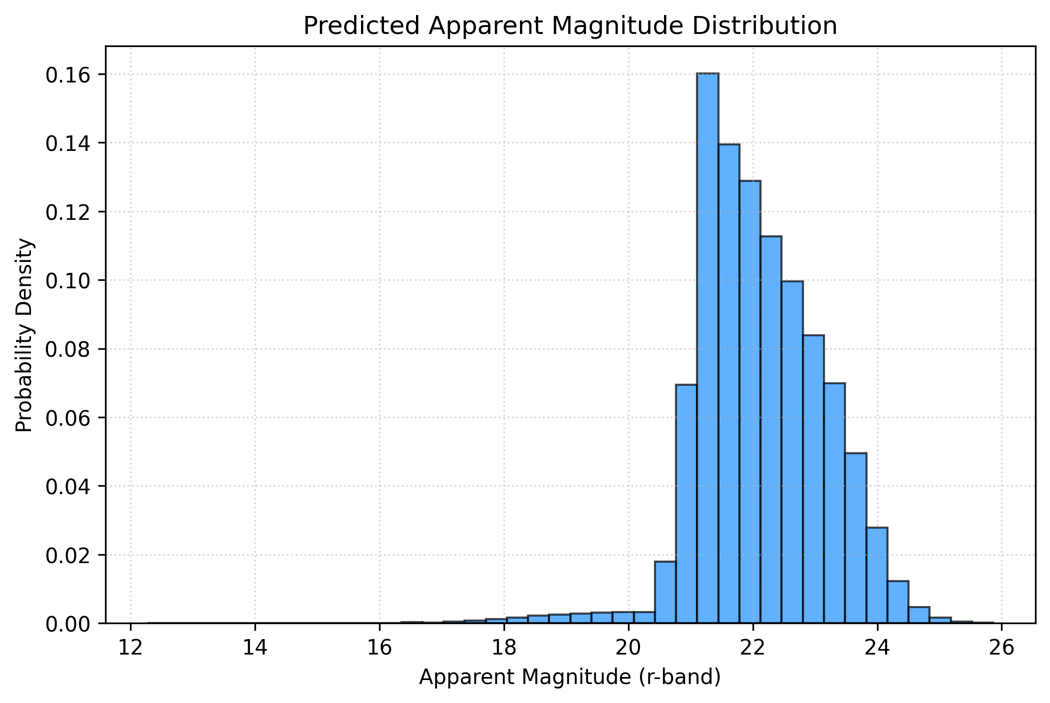Figure 1. Prior-weighted distribution of predicted r-band apparent magnitude. The bulk lies between 21 and 24, with the faint tail (m_r > 24.5) representing the hardest-to-detect orbits.

6.2 Where to look

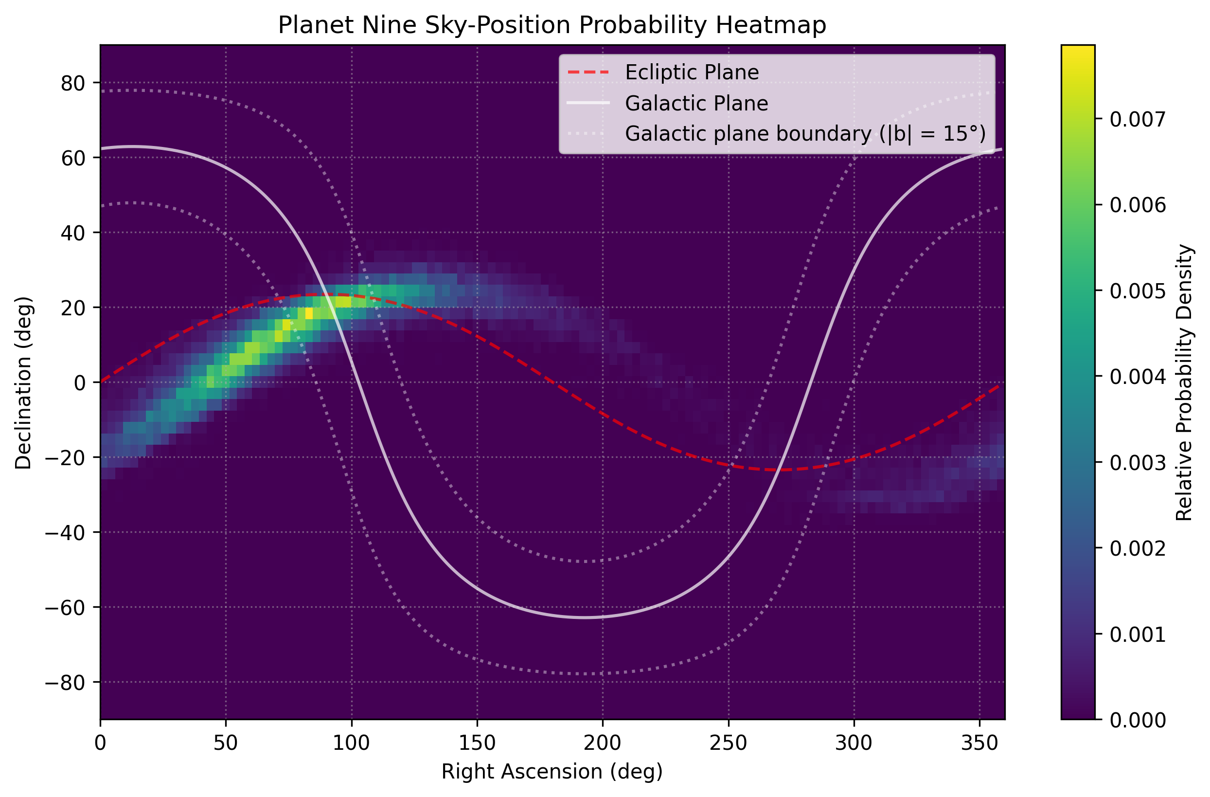Figure 2. On-sky probability density (geocentric equatorial). The highest-probability region follows the ecliptic and concentrates in the northern winter sky, roughly RA 3h–6h, Dec +10° to +30° — the aphelion direction where a body on an eccentric orbit spends most of its time. The white curves mark the galactic plane and its |b| = 15° confusion zone, where stellar crowding suppresses detection.

The probability mass tracks the ecliptic (as expected for a planet) and piles up toward aphelion. Where that arc crosses the galactic plane, detection is degraded — a real observational handicap, not a modelling artifact.

6.3 Sensitivity: what drives the uncertainty

| Driver | Raw Pearson $r$ with $m_r$ | Interpretation | | :--- | ---: | :--- | | Heliocentric distance $d$ | +0.95 | Dominant. Sets brightness via $d^{-4}$. | | Semi-major axis $a$ | +0.75 | Drives $d$, hence correlated. | | Eccentricity $e$ | +0.33 | Modulates current $d$ given phase. | | Radius $R$ | +0.24 | Weak; mass–radius scaling is shallow. | | Albedo $p_V$ | −0.09 | Near-zero raw — see note. |

To visualize how the orbital inclination parameters affect the detection probability across the LSST survey masks, run the simulation below:

On the albedo result. The near-zero raw correlation is not a bug and not evidence that albedo is irrelevant. Albedo enters $H_V$ directly and spans ~0.55 mag across the sampled range, but heliocentric distance varies so much more that it dwarfs albedo in an unconditioned correlation. Holding distance and radius fixed, the partial correlation of albedo with $m_r$ is −0.998 — i.e. at fixed distance, albedo almost entirely determines the residual brightness, exactly as the physics requires. The lesson is that distance uncertainty must be reduced before albedo matters observationally, not that albedo is unimportant.

6.4 When, and by which instrument

Detection year is modelled per facility:

• Vera C. Rubin Observatory / LSST (10-yr survey; $\delta \le +15°$, $m_r < 25.0$): bright targets ($m_r < 23.5$) found in the first 1–2 seasons; mid-range by years 3–5; the faintest ($24.5 \le m_r < 25$) only via multi-year shift-and-stack. Galactic-plane samples carry a 70% per-pass miss penalty.
• Subaru / Hyper Suprime-Cam (targeted deep fields, $m_r < 26.0$): covers the aphelion box (RA 2.5h–5.5h, Dec +5° to +25°) with ~80% completeness outside the galactic plane, ~30% inside, on a 2026–2029 timescale.
• Infrared (archival IRAS/AKARI plus NEO Surveyor): models thermal detection for $d_{\text{hel}} < 450$ AU on a 2028–2033 window. Note: NEO Surveyor's operational dates should be reconfirmed against the current mission baseline before this window is cited as firm.

The combined curve takes the earliest detection across facilities.

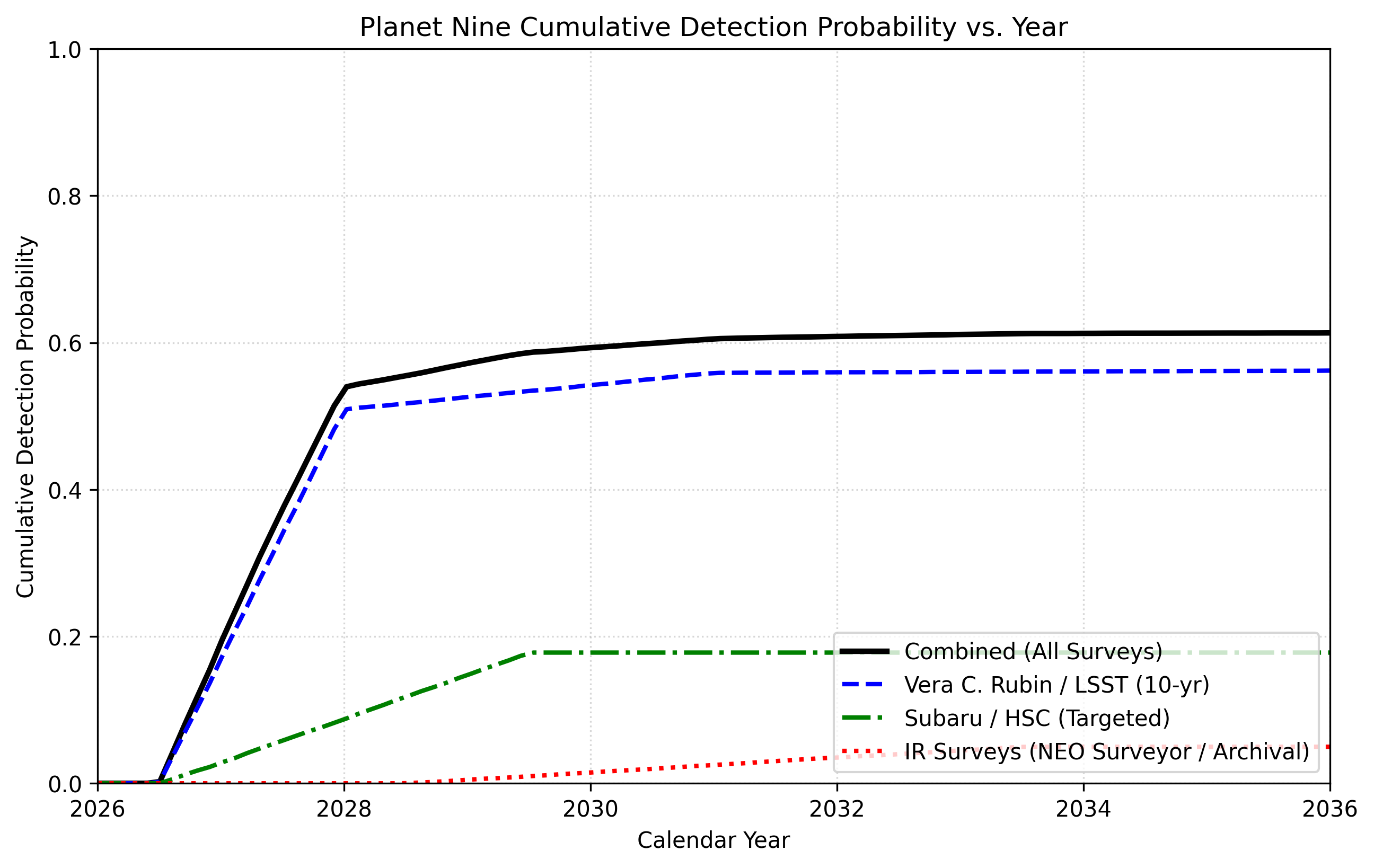Figure 3. Cumulative detection probability by year. The combined probability (black) climbs steeply as LSST reaches depth and asymptotes near 0.61 around 2030. LSST (blue) is the dominant contributor; Subaru/HSC (green) and IR surveys (red) add smaller increments.

The combined cumulative probability reaches ~61% by 2030 and then flattens. The residual ~39% corresponds to orbits that are simultaneously too faint ($m_r > 25$) and outside the deep targeted footprints — the parameter space that a future ≥10 m-class facility would be needed to close.

7. If nothing is found: the null-detection posterior

Treating existence as uncertain, we start from a stated prior $P(\text{exists}) = 0.70$ and apply Bayes' rule given continued non-detection. With $P(\text{null} \mid \text{exists}) = 1 - P_{\text{combined}}(\le \text{year})$ and $P(\text{null} \mid \text{not exists}) = 1$:

$P(\text{exists} \mid \text{null}) = \frac{P(\text{null}\mid\text{exists})\,P(\text{exists})}{P(\text{null}\mid\text{exists})\,P(\text{exists}) + 1\cdot(1-P(\text{exists}))}$

| Through end of | $P(\text{detect}\mid\text{exists})$ | Posterior $P(\text{exists}\mid\text{null})$ | | :--- | ---: | ---: | | 2026 | ~0% | 70.0% | | 2028 | ~54% | 51.8% | | 2030 | ~59% | 48.7% | | 2036 | ~61% | 47.4% |

A decade of LSST silence would pull the posterior from 70% down toward ~47% — substantial erosion, but not refutation, precisely because ~39% of the orbit stays beyond reach. The hypothesis is hard to kill with these instruments even though it is reasonably easy to confirm if the planet sits in the favorable bright/accessible region.

8. Limitations and open questions

• Existence is unproven. Everything here is conditional. The clustering signal is statistically suggestive but contested, and observational bias remains a live alternative explanation.
• Distance dominates everything. The single largest lever on detectability is the planet's current heliocentric distance, which the data constrain only weakly. Until that tightens, brightness predictions carry a wide spread and secondary parameters (albedo, radius) cannot be observationally isolated.
• The detection blind spot is structural. The ~39% residual is not pessimism about LSST but a real consequence of the faint, distant tail; closing it requires a ≥10 m-class survey capability.
• Detection-timing model is heuristic. Per-facility detection years are drawn from plausible binned schedules, not a cadence-level survey simulator (e.g. Sorcha/rubin_sim). A full opsim-based treatment would refine the CDF shape.
• Mass–radius relation is a placeholder. $R \propto \sqrt{M}$ is a convenience scaling, not a calibrated relation.
• NEO Surveyor schedule needs reconfirmation against the current mission baseline.
• Static epoch. Positions are evaluated at a single date; parallax motion over a survey baseline (a key real-world discriminator) is not modelled dynamically.

9. Reproducibility

All results derive from a single script, simulation.py (N = 100,000, numpy seed 42), using numpy, astropy, and matplotlib. The script samples the ensemble, propagates orbits, applies survey masks, and emits the three figures and all printed credible intervals, correlations, and posteriors.

The script, the three output figures, and dependency/run instructions are available at: https://github.com/Maha-Strategies/planet-nine-forecast

References

• Batygin, K., Adams, F. C., Brown, M. E., & Becker, J. C. (2019). The Planet Nine Hypothesis. Physics Reports, 805, 1–53. arXiv:1902.10103.
• Brown, M. E., & Batygin, K. (2021). The Orbit of Planet Nine. The Astronomical Journal. arXiv:2108.09868.
• Brown, M. E., & Batygin, K. (2016). Observational Constraints on the Orbit and Location of Planet Nine in the Outer Solar System. arXiv:1603.05712.
• Batygin, K., & Brown, M. E. (2016). Evidence for a Distant Giant Planet in the Solar System. The Astronomical Journal.
• Siraj, A., Chyba, C. F., & Tremaine, S. (2025). Orbit of a Possible Planet X. The Astrophysical Journal, 978, 139. https://doi.org/10.3847/1538-4357/ad98f6
• Vera C. Rubin Observatory / LSST documentation, Rubin Observatory.
• NSF–DOE Vera C. Rubin Observatory first-imagery release (2025).
• Reproducibility repository (simulation code and figures): https://github.com/Maha-Strategies/planet-nine-forecast

Citations are provided for traceability. The Siraj et al. (2025) parameters (ApJ 978, 139) and the Batygin et al. (2019) ranges (Physics Reports 805, 1–53) have been confirmed against their primary publications. The Brown & Batygin (2021) semimajor-axis distribution is consistent with the cited orbit paper (AJ); the author should confirm the exact volume/DOI matches the specific 2021 paper the [b] parameters were drawn from. The NEO Surveyor operational window should be reconfirmed against the current mission baseline before that detection window is cited as firm.